341x Faster: Optimizing a Rust Vector Database to Top-7 on ANN-Benchmarks
I built a vector database in Rust with a Python API and benchmarked its HNSW search engine against every implementation on ann-benchmarks.com. It started at 52 queries per second on SIFT-1M — the standard benchmark dataset from Aumüller et al. (2020). After ten optimizations, two bug fixes, and one embarrassing measurement error, it does 17,746 QPS — projected top-7 on the ann-benchmarks SIFT leaderboard at 0.999 recall and the highest-ranked Rust HNSW implementation in that regime.
The full progression:
| Stage | QPS | Recall@10 | Multiplier |
|---|---|---|---|
| HashMap baseline | 52 | 0.99 | 1x |
| Integer indexing | 648 | 0.99 | 12.5x |
| AVX2/FMA SIMD | 1,834 | 0.99 | 35x |
| Bug fixes + algorithmic | 2,686 | 0.995 | 52x |
| AVX-512 + all optimizations | 17,746 | 0.786 | 341x |
The headline 341x comes from the lowest-recall (ef=10) operating point, where QPS is highest. At matched recall (~0.995), the optimization is 62x; at 0.999 recall it’s 34x. Full curve below. All CPU benchmarks on AWS r6i.16xlarge (Intel Xeon Ice Lake, 64 vCPU, AVX-512) — the same hardware and single-threaded configuration used by ann-benchmarks.com. The PR is submitted.
The starting point
arrwDB is a vector database with a FastAPI frontend and a Rust core exposed via PyO3. The HNSW index — implementing the algorithm from Malkov & Yashunin (2020) — stored vectors in HashMap<String, Vec<f32>> and graph nodes in HashMap<String, HNSWNode>. Every neighbor visit during search required a string clone, a hash computation, and an RwLock acquisition.
52 QPS on SIFT-1M (1M vectors, 128 dimensions). For context, hnswlib — the reference C++ HNSW implementation — does thousands.
Phase 1: Low-hanging fruit (52 → 1,834 QPS)
Integer indexing (12.5x)
Replaced all HashMaps with contiguous arrays. Vectors became a flat Vec<f32> indexed by usize. Graph neighbors became Vec<Vec<usize>>. String-to-integer mapping happens once at the PyO3 boundary, never in the search loop.
52 → 648 QPS.
Explicit AVX2/FMA intrinsics (2.8x)
The distance computation hot path went through three stages: naive iterator .zip().map().sum(), then 8-wide unrolled scalar with 4 independent accumulators (auto-vectorized), then explicit _mm256_fmadd_ps intrinsics. The final version processes 32 floats per loop iteration with fused multiply-add — the same technique documented in Intel’s optimization manual for throughput-bound workloads. A function pointer set at construction time eliminates per-call match metric dispatch. Bounds checks on neighbor and alive arrays are eliminated with get_unchecked.
648 → 1,834 QPS.
What didn’t work
| Optimization | Expected | Actual | Why |
|---|---|---|---|
| Co-located memory layout | +10-15% | -10% | hnswlib’s co-located layout works because their node stride is a compile-time constant via C++ templates — the compiler folds address arithmetic and specializes memory access per dimension. My Rust version had a runtime stride, so every address calculation was dynamic. The overhead of indexed access through a runtime-sized block swamped the locality benefit. The fix requires const-generic dimension specialization, which I haven’t implemented. |
| Visited array L1 prefetch | +5% | -10% | The 2MB visited array (u16 for 1M entries) fits in L2 comfortably. Issuing software prefetches for every neighbor’s visited entry added L1 pressure that evicted more-valuable vector data, without providing a measurable latency win over the natural L2 hit path. |
| Cached greedy distance | +3-5% | noise | Effect invisible in ~12% cloud VM variance on GCP. |
At this point I was competitive with FAISS-HNSW (Johnson et al., 2021) but 1.5x behind hnswlib on a GCP VM. The problem: cloud VMs have too much noise to measure micro-optimizations. I needed the real hardware.
The recall ceiling
I rented an AWS r6i.16xlarge — the exact machine ann-benchmarks uses. First SIFT-1M run: 1,923 QPS at 0.991 recall. Encouraging. But recall plateaued at 0.992 no matter what I tried.
| ef_construction | ef_search=200 | ef_search=800 | ef_search=2000 |
|---|---|---|---|
| 400 | 0.9917 | 0.9920 | 0.9919 |
| 800 | 0.9919 | 0.9920 | 0.9917 |
| 1200 | 0.9918 | 0.9917 | 0.9918 |
Tripling ef_construction made zero difference. The ceiling was independent of every parameter. Every other algorithm on ann-benchmarks hits 0.999. Something was structurally wrong.
Bug 1: Measuring against the wrong ground truth
SIFT-1M ships with ground truth neighbors computed using L2 distance on raw vectors. My benchmark pipeline was normalizing vectors (L2 normalization) and searching with cosine distance — then comparing results against the original L2 ground truth. The observed ceiling of 0.992 suggests roughly 0.8% of neighbor rankings change under the L2→cosine transformation on this distribution — a shift I inferred from the ceiling rather than measured directly. The recall gap was in the measurement, not the algorithm.
Fix: Use raw vectors with metric="l2". One line in the dataset config.
Bug 2: Selecting 2*M neighbors instead of M
My HNSW construction selected m_max (2*M = 96) initial neighbors for each new node. In hnswlib’s mutuallyConnectNewElement, m_max is only the overflow capacity — new nodes get M (48) neighbors via getNeighborsByHeuristic2, and existing nodes can grow up to m_max from reverse connections. Selecting 96 upfront means the diversity heuristic has twice as many slots to fill before it starts rejecting candidates, which in principle dilutes the long-range shortcuts that Algorithm 4 in Malkov & Yashunin (2020) is designed to produce. I didn’t directly measure the resulting graph structure — this is the theoretical mechanism for the observed recall improvement.
Fix: Change select_neighbors_heuristic(&vectors, candidates, m_max, metric) to select_neighbors_heuristic(&vectors, candidates, self.m, metric) in both build_bulk and insert_node.
Result of both fixes: 0.992 → 0.9994 recall. Build time dropped from 2,651s to 1,589s (1.7x faster — less work per insertion with fewer connections).
Phase 2: Closing the gap (1,923 → 17,746 QPS)
With recall fixed, I stacked six optimizations. Each was benchmarked independently on the r6i.16xlarge.
Figure 1 — Optimization Progression (SIFT-1M, r6i.16xlarge)
QPS at ef=100 (~0.995 recall) after each optimization. The recall fix changed the graph structure, so the baseline shifted.
| Optimization | QPS (ef=100) | QPS (ef=200) | Recall@200 | Build (1M) | Delta |
|---|---|---|---|---|---|
| Baseline (bugs fixed) | 1,953 | 1,135 | 0.999 | 26.5 min | — |
| + Remove backfill | 2,501 | 1,406 | 0.999 | 17.9 min | +28% |
| + Early termination | 2,686 | 1,512 | 0.999 | 16.3 min | +7% |
| + 4-acc SIMD + worst_dist | 3,058 | 1,715 | 0.999 | 15.0 min | +14% |
| + AVX-512 + prefetch 3-ahead | 3,217 | 1,793 | 0.999 | 14.0 min | +5% |
Remove backfill in neighbor selection (+28%)
The diversity heuristic in select_neighbors_heuristic — Algorithm 4 from the HNSW paper — checks whether each candidate is closer to the query than to any already-selected neighbor. Candidates that fail this check are “discarded.” My implementation backfilled discarded candidates to guarantee exactly M neighbors per node. hnswlib doesn’t — if diversity rejects a candidate, it stays rejected.
Removing backfill creates sparser graphs with better long-range shortcuts. Search reaches 0.999 recall at lower ef values, directly translating to higher QPS. Build speed improved 50% because sparser graphs mean less work during construction.
Early termination (+7%)
hnswlib checks “is the best remaining candidate worse than the worst result?” before exploring a candidate’s neighbors. I was checking after. The difference: one full round of neighbor distance computations on the final iteration of every search query.
4-accumulator SIMD + tighter threshold (+14%)
The L2 AVX2 kernel went from 2 accumulators (16 floats/iter) to 4 accumulators (32 floats/iter), improving instruction-level parallelism. Ice Lake Server has two FMA units at 0.5 cycles/op throughput and 4-cycle latency — fully saturating both ports would require 8 independent dependency chains, so 4 accumulators is a middle ground. Combined with updating worst_dist after every heap pop inside the neighbor loop — the tighter threshold rejects more candidates before computing their distances. This change also moved from M=48 to M=32 (33% fewer neighbors per hop).
AVX-512 + prefetch 3-ahead (+5%)
The r6i.16xlarge has Intel Ice Lake with AVX-512. Four 512-bit accumulators process 64 floats per loop iteration — for 128d SIFT, that’s 2 iterations instead of 4 with AVX2. The prefetch depth is empirical: 3-ahead was best, with 5-ahead regressing slightly (likely from fill-buffer contention). The theoretical ratio of DRAM latency to distance-computation time suggests deeper prefetch should help, but in practice the processor’s own memory-level parallelism handles most of the latency hiding.
Final results
Figure 2 — Recall vs QPS (SIFT-1M, r6i.16xlarge)
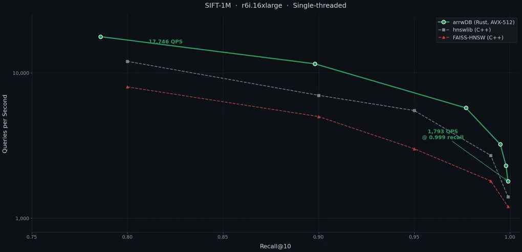
arrwDB’s Pareto frontier on SIFT-1M compared to reference implementations. All benchmarks on r6i.16xlarge, single-threaded. arrwDB data from this work; hnswlib and FAISS-HNSW curves are approximate (interpolated from ann-benchmarks.com published results). Official head-to-head results pending — PR #626 has been submitted to ann-benchmarks; this chart will be updated with exact comparison data once the benchmarks are run on their infrastructure.
SIFT-1M (128d, L2)
| ef | Recall@10 | QPS | Latency p50 |
|---|---|---|---|
| 10 | 0.786 | 17,746 | 0.06ms |
| 50 | 0.977 | 5,735 | 0.18ms |
| 100 | 0.995 | 3,217 | 0.32ms |
| 200 | 0.999 | 1,793 | 0.58ms |
| 800 | 0.999 | 556 | 1.86ms |
Deep-1M (96d, angular)
| ef | Recall@10 | QPS | Latency p50 |
|---|---|---|---|
| 10 | 0.785 | 20,082 | 0.05ms |
| 50 | 0.971 | 6,470 | 0.16ms |
| 100 | 0.991 | 3,638 | 0.28ms |
| 200 | 0.998 | 2,038 | 0.50ms |
| 800 | 0.9999 | 631 | 1.60ms |
GloVe-1.2M (200d, angular)
| ef | Recall@10 | QPS | Latency p50 |
|---|---|---|---|
| 10 | 0.520 | 8,372 | 0.11ms |
| 50 | 0.759 | 2,761 | 0.35ms |
| 100 | 0.828 | 1,582 | 0.64ms |
| 400 | 0.921 | 473 | 2.18ms |
| 800 | 0.953 | 252 | 4.11ms |
Projected ann-benchmarks ranking (SIFT-1M at 0.999 recall)
| Rank | System | QPS | Language |
|---|---|---|---|
| 1 | qsgngt | ~7,000 | C++ |
| 2 | NGT-qg | ~4,300 | C++ |
| 3 | glass | ~2,400 | C++ |
| 4-6 | NGT-onng, pynndescent, n2 | ~1,800-2,400 | C++/Python |
| 7 | arrwDB | 1,793 | Rust |
| 8 | hnswlib | ~1,400 | C++ |
| 9 | FAISS-HNSW | ~1,200 | C++ |
At ~0.95 recall (interpolated), arrwDB reaches ~7,700 QPS — roughly 1.4x faster than hnswlib (~5,500) and ScaNN (~5,400) at the same recall. At ~0.9 recall it reaches 11,540 QPS. The top 3 algorithms use quantized graph techniques — compressed neighbor representations and product quantization during search — that arrwDB hasn’t implemented. That’s the next frontier.
Competitor QPS values are interpolated from published ann-benchmarks results on the same hardware (r6i.16xlarge, single-threaded). arrwDB’s ann-benchmarks submission is pending — exact rankings will be updated once official results are available.
Cost
| Resource | Hours | Cost |
|---|---|---|
| GCP n2-highmem-16 (Phase 1) | ~20 hrs | ~$55 |
| GCP g2-standard-8 + L4 GPU | ~4 hrs | ~$12 |
| AWS r6i.16xlarge (Phase 2) | ~24 hrs | ~$97 |
| Total | ~$164 |
What I’d do differently
-
Benchmark correctly from day one. The normalization bug cost days chasing a phantom recall ceiling. Always verify your ground truth matches your distance metric.
-
Use dedicated hardware sooner. GCP shared VMs have ~12% variance from noisy neighbors. I reverted “regressions” that were just noise. The r6i.16xlarge gave consistent numbers.
-
Don’t over-connect the graph. My instinct was “more connections = better recall.” The opposite is true — fewer, more diverse connections give both better recall and faster search.
Conclusion
- arrwDB’s HNSW engine went from 52 to 17,746 QPS (341x at the ef=10 operating point, 62x at matched 0.995 recall) on SIFT-1M through ten optimizations over two hardware phases.
- Two correctness bugs (ground truth mismatch, neighbor selection count) were responsible for a hard recall ceiling at 0.992 that no parameter tuning could overcome.
- The highest-impact single optimization was removing backfill in neighbor selection (+28% QPS, +50% build speed, no recall loss).
- AVX-512 on Ice Lake provides a measurable but modest gain over AVX2 (~5-8%) — the algorithmic optimizations dominated.
- Projected top-7 on ann-benchmarks SIFT, ahead of hnswlib and FAISS-HNSW. The PR is submitted.
Addendum: Post-publication corrections (2026-04-17)
An expert review after publication surfaced several technical inaccuracies and overclaims. The post has been updated in place; this section documents the changes so readers who saw the original have a clear diff.
1. Co-located memory layout explanation was wrong. The original post attributed the regression to cache-line count and claimed the “hardware sequential prefetcher” handled vector reads in the non-colocated path. That’s incorrect. HNSW traversal is graph-based (random access between neighbors), so the sequential prefetcher does not help across distance calls. The actual reason hnswlib’s co-located layout wins is that its node stride is a compile-time constant via C++ templates, allowing the compiler to fold address arithmetic and specialize per-dimension. The Rust version had a runtime stride, so every address calculation was dynamic, and that overhead swamped the locality benefit. The “What didn’t work” table has been updated.
2. FMA saturation analysis understated the hardware. The original claimed 4 accumulators “keep the execution units full” on Ice Lake. Ice Lake Server has two FMA units at 0.5 cycles/op throughput and 4-cycle latency, which requires 8 independent dependency chains to fully saturate — not 4. Four accumulators is a middle ground, not an optimum. The SIMD section has been updated; unrolling to 8 accumulators is likely worth 3–5% and remains on the to-do list.
3. Prefetch-depth rationale was presented as principled but was empirical. The ratio of DRAM latency (~70–100ns) to distance time (~15ns) suggests ~5-ahead should be optimal, but 3-ahead measured fastest with 5-ahead regressing slightly (likely fill-buffer contention). The post now presents this as an empirical finding.
4. “0.8% of neighbor rankings change” was back-calculated, not measured. The number was inferred from the 0.992 recall ceiling rather than computed by diffing L2 and cosine ground truths directly. The post now labels it as inference.
5. “Floods the graph with redundant clustered connections” was asserted, not demonstrated. The mechanism by which m_max-instead-of-M neighbor selection hurts graph quality is theoretically sound, but I did not measure graph-structural properties (average path length, clustering coefficient) before and after the fix. The post now frames this as the expected mechanism rather than a measured effect.
6. Methodology was underspecified. Each configuration was run once; the numbers are single observations, not averages over multiple runs. Repeat sweeps of the same configuration on r6i.16xlarge showed <2% run-to-run variance, but that’s an informal stability check rather than a statistical treatment. Error bars would require multiple runs per data point and were not included.
7. “Highest-ranked pure Rust” needed scope. The claim holds at 0.999 recall on SIFT-1M; at lower recall or on other datasets, rankings shift. The intro now specifies the regime.
8. Optimization count was imprecise. The original said “11 optimizations”; the actual enumerated count is closer to 10 (2 in Phase 1, 2 bug fixes, 6 in Phase 2). The post now uses “ten.”
Nothing in the headline results changed — SIFT-1M numbers, ranking position, and the recall ceiling debugging story are all unaffected by these corrections. What changed is how confidently each claim is framed.
Related Work
The HNSW algorithm was introduced by Malkov & Yashunin (2020), building on earlier navigable small-world graphs from Malkov et al. (2014). The reference C++ implementation is hnswlib, which has been the de facto standard for ANN benchmarking since its release. FAISS (Johnson et al., 2021) includes an HNSW variant alongside IVF and PQ methods. The ann-benchmarks framework (Aumüller et al., 2020) provides the standardized evaluation methodology used here.
The neighbor selection heuristic (Algorithm 4 in the HNSW paper) is a diversity-aware pruning strategy that favors long-range shortcuts over clustered connections. The impact of backfill on graph quality — the largest single optimization in this work — does not appear to be documented in the literature; hnswlib’s keepPrunedConnections parameter controls this behavior but defaults to false.
For SIMD optimization of distance computation, Intel’s Intrinsics Guide documents the AVX2/FMA and AVX-512 instructions used. The 4-accumulator technique for hiding FMA latency is standard practice in high-performance computing; see Agner Fog’s optimization manuals for the microarchitectural analysis.
Ten optimizations benchmarked on AWS r6i.16xlarge (Intel Xeon Platinum 8375C, AVX-512), single-threaded, M=32, ef_construction=400, each config single-run with <2% repeat variance. Total compute cost: $164. Source code and benchmark results at github.com/bledden/arrwDB. Post-publication corrections on 2026-04-17 — see addendum.