Adapting Noisy Student to the LLM Era: Four Experiments in Self-Training
A Proposal and a Simple Idea
Noisy student self-distillation (Xie et al., 2020) got state-of-the-art on ImageNet by iteratively training student models on teacher-generated pseudo-labels with noise augmentation. The key mechanism: noise (RandAugment, dropout, stochastic depth) regularized the student, preventing overfitting to potentially incorrect pseudo-labels. The obvious next step was to try this with LLMs.
The Thinking Machines Lab proposal asked a specific question: could this technique bootstrap limited labeled data into effective utilization of larger unlabeled datasets, using reinforcement learning with verifiable rewards (RLVR)? Unlike image classification, many language tasks offer automatic verification - code can be executed against test cases, math answers can be checked. This meant pseudo-labels could be verified, not just guessed.
I set up on the Tinker API with Qwen/Qwen3-30B-A3B-Instruct-2507 (30B parameters, 3B active via MoE), fine-tuned with LoRA rank 32. The plan was to start with the simplest possible transfer of the noisy student recipe to language and iterate from there.
I didn’t anticipate that “iterate from there” would mean four redesigns, a severe overfitting crisis, an 8% baseline that needed forensic investigation, and billing exhaustion right when the most interesting results were starting to show up.
V1: Porting Token Noise from Vision (It Didn’t Work)
The first attempt was the most direct translation possible: take the noisy student recipe, replace pixel augmentation with token-level dropout, and see what happens. I used a 30B teacher to pseudo-label 50 code generation prompts, then trained a 4B student on those labels with and without noise. The noise configuration was 10% activation dropout plus 10% input token dropout - randomly removing tokens from the training prompt before tokenization.
I ran 10 seeds per condition. The results came back fast and were clear-cut.
WandB Training Curves (view project): The V1 train/loss panels show all 20 runs (10 seeds × 2 conditions) descending sharply from ~2,000 to ~500 within the first 10 steps, then stabilizing. The noise condition runs consistently settle at higher final loss values with visibly wider spread between seeds. The train/confidence panel - tracking reward model confidence - rises from 0.20 to 0.35 over the 40-step training window, with the no-noise runs reaching higher peak confidence. The separation between conditions is evident in both metrics, consistent with the p=0.0018 statistical result.
Token-level noise didn’t just fail to help - it actively hurt training, with a large effect size (g=1.57) and double the variance. In hindsight this makes sense: a flipped photo of a cat is still recognizably a cat, but "Write a function to calculate Fibonacci numbers" with tokens dropped becomes "Write function calculate" - gibberish. Image augmentations stay on the data manifold. Token dropout doesn’t.
The lesson that shaped everything after: The noisy student mechanism works because noise regularizes without destroying meaning. For language, meaning is too densely packed in every token for dropout-style perturbation. If noise was going to play a role, it would have to come from somewhere else entirely.
This negative result took about 8 GPU-hours and ~$6. Cheapest experiment of the project, and probably the most important - it killed the simplest adaptation path and forced a full redesign.
V2: Redesign, Overfitting, and Debugging
V1 failing forced me to rethink the whole approach. Instead of injecting noise explicitly, what if the natural variance of language model sampling - generating diverse outputs at temperature 0.7 - served as the “noise”? And instead of relying on teacher confidence to filter pseudo-labels, what if I verified them? Code can be executed. Math answers can be checked. That became V2: replace explicit noise with sampling variance, replace teacher confidence with automatic verification, replace distillation with RLVR.
The algorithm was simple in theory:
For each iteration i = 0, 1, ..., N-1:
  1. Train model with RL on current dataset (RLVR with verifiable rewards)
  2. Generate K=8 samples for each unlabeled problem (consensus sampling)
  3. Verify samples against ground truth (code execution or answer matching)
  4. Accept pseudo-labels where ≥1 of 8 samples is correct
  5. Merge labeled data with accepted pseudo-labels for next iteration
Following the original proposal’s step 4, the implementation relabels the entire unlabeled pool each iteration using the improved model - not just the newly added data. In practice, with pseudo-label acceptance already above 93%, relabeling changed very little: the improved model accepted a few more problems (e.g., 4,685 → 4,714 in the scarcity run) but the overall composition was nearly identical. Pseudo-labeling is skipped on the final iteration since no further training follows.
The Overfitting Wall
The first V2 runs produced alarming results: training pass rate hit 87-100%, but evaluation pass@1 sat at 9-14%. The model was memorizing the training data perfectly while learning nothing generalizable. Even worse, pseudo-labeling accepted only 6 out of 120 problems (5%) - the pipeline was starving itself of training signal.
This turned out to be a multi-parameter problem. The original hyperparameters from the V1 experiment (learning rate 1e-5, no weight decay, confidence threshold 0.5) were all wrong for RLVR self-training. RL gradients are noisier than supervised gradients, so the model overfit faster. The confidence threshold of 0.5 required that at least 4 of 8 consensus samples be verified-correct - far too strict for bootstrapping. It took several debugging cycles to identify and fix all four problems simultaneously:
| Change | From | To | Rationale |
|---|---|---|---|
| Learning rate | 1e-5 | 5e-6 | RL gradients are noisy; slower learning prevents overfitting |
| Confidence threshold | 0.5 | 0.125 | 0.5 requires ≥4/8 correct - too strict for early-stage models |
| Weight decay | 0.0 | 0.01 | L2 regularization |
| Early stopping | None | Patience=5 | Halt training before regression sets in |
The confidence threshold was the big one. Lowering it from 0.5 to 0.125 (accepting a pseudo-label if at least 1 of 8 samples is correct) massively increased pseudo-label yield while still guaranteeing every accepted example had at least one verified-correct solution. This was the difference between a self-training pipeline that starves and one that feeds itself.
First Try: Code Generation (The 8% Wall)
With the overfitting resolved, I ran the full V2 pipeline on MBPP code generation - 164 labeled problems, 374 unlabeled, 3 iterations. The result: 8% baseline pass@1, only 25 pseudo-labels generated (3.5% acceptance), +1% improvement.
Something was wrong with the baseline. I dug into it - re-evaluated all 13 accepted pseudo-labeled examples against original test cases, looked at model output patterns, and checked the code extraction logic. The investigation (documented in CODE_BASELINE_INVESTIGATION.md) turned up three compounding factors:
- Verbose multi-language outputs: The model generated comprehensive “educational” responses with Python, JavaScript, and Java implementations, blowing through the 512-token limit.
- Truncation: 92.3% of responses were cut off mid-function, producing non-executable code.
- Function name mismatches: MBPP tests assert against specific names like
remove_Occ, but the model generatedremoveOccurrenceorremove_occurrence.
The pseudo-labeling system itself was working fine - all 25 accepted labels passed verification. The problem was that the model just couldn’t produce correct code often enough to generate training signal. At 3.5% acceptance, the self-training loop had almost nothing to learn from.
Pivoting to Math: Where Self-Training Actually Worked
The code results raised the obvious question: was the self-training approach broken, or was it just the wrong task? Math reasoning on GSM8K was a good test - same model, same pipeline, same hyperparameters, but a task where the model was already competent (84% baseline vs 8%).
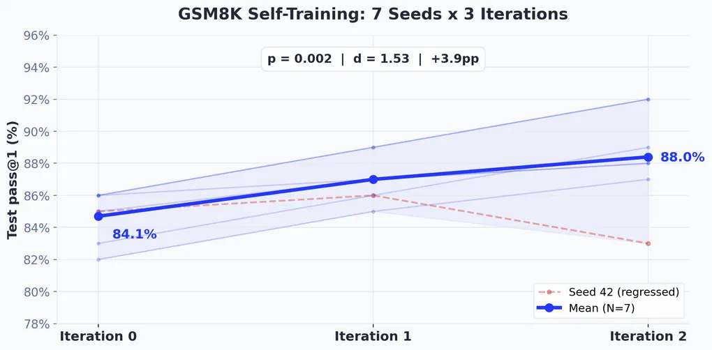
I ran 7 seeds (42-48) with 3 iterations per seed. The contrast with code was stark.
Per-Seed Results
| Seed | Initial pass@1 | Final pass@1 | Δ | Best eval |
|---|---|---|---|---|
| 42 | 85% | 83% | −2% | 94% |
| 43 | 82% | 87% | +5% | 92% |
| 44 | 86% | 92% | +6% | 94% |
| 45 | 85% | 88% | +3% | 96% |
| 46 | 86% | 88% | +2% | 94% |
| 47 | 83% | 89% | +6% | 94% |
| 48 | 86% | 92% | +6% | 94% |
WandB Iteration Metrics (view report): The V2 dashboard tracks all 9 runs (7 math seeds + 2 scarcity seeds) across three iteration panels. The iter0/test_pass@1 chart shows math seeds clustered tightly between 0.82-0.86, with the two scarcity runs (L10) at 0.83 and 0.87. By iter2/test_pass@1, the spread widens: most math seeds reach 0.87-0.92, while the scarcity L10/seed42 run hits 0.92 at the top. The pseudo_labels panels reveal the starkest difference - math runs generate ~350 pseudo-labels per iteration (flat bars), while the scarcity runs produce 4,600-4,700 (dominant bars dwarfing the rest), reflecting the 13× larger unlabeled pool. The pseudo_label_rate panels show both conditions achieving >93% acceptance, confirming pseudo-label quality is consistent regardless of pool size.
Six of seven seeds improved. The one that didn’t - seed 42, which regressed 2% despite hitting 94% during training - is why running multiple seeds matters. A single-seed experiment could have told a completely different story.
Pseudo-Labeling Statistics
| Metric | Mean | Range |
|---|---|---|
| Acceptance rate | 93.6% | 91-96% |
| Average confidence | 0.94 | 0.93-0.96 |
| Pseudo-labels per iteration | ~350 | 341-359 |
| Total pseudo-labels per seed | ~700 | 686-715 |
The Bootstrap Threshold
The contrast between math and code told a clear story. Putting them side-by-side made the pattern obvious:
Self-training is a bootstrapping technique - it amplifies existing capability but can’t create it from nothing. When the model already solves most problems (84% on math), consensus pseudo-labeling floods the pipeline with high-quality training data. When it rarely produces correct solutions (8% on code), the pipeline starves. I’d estimate the practical threshold at roughly 60-80% baseline pass@1, though the exact boundary depends on the task.
Most improvement came in iterations 0 and 1. Iteration 2 sometimes caused regression, which points to diminishing returns and overfitting risk from extended self-training. The best eval scores during training (92-96%) consistently exceeded final test performance (83-92%), suggesting some distribution shift between training/evaluation and held-out test data.
Data Scarcity: The Most Interesting Question, Cut Short
After the math results came in, I realized V2 hadn’t actually tested what the original proposal asked for. The proposal was about bootstrapping limited labeled data. V2 used 164 labeled examples - a moderate amount - paired with only 374 unlabeled problems. That’s a 2.3× expansion ratio. Not exactly “limited labeled data, large unlabeled pool.”
I designed a V3 scarcity experiment to test the real question: does self-training help more when labeled data is genuinely scarce? Five conditions (10, 20, 50, 100, 164 labeled examples), each with 5,000 unlabeled problems, across 5 seeds each - 25 total runs.
H1: Self-training improvement correlates negatively with labeled data availability - less labeled data yields proportionally greater benefit from self-training.
Billing ran out on the Tinker platform. Only 1 of 25 planned runs completed fully (L10/seed42), with a second run partially completing (L10/seed43, 2 of 3 iterations). The remaining 23 runs died immediately with HTTP 402 errors.
But that one complete run produced the most surprising result of the project.
Complete Run: L10, Seed 42
| Iteration | Training data | Best eval | Test pass@1 | Pseudo-labels | Acceptance |
|---|---|---|---|---|---|
| 0 | 10 | 90% | 87% | 4,685 / 5,000 | 93.7% |
| 1 | 4,695 | 94% | 90% | 4,714 / 5,000 | 94.3% |
| 2 | 4,724 | 96% | 92% | - (final) | - |
The baseline was way higher than expected. I expected 10 labeled examples to produce a ~30-40% baseline. Instead: 87%. Qwen3-30B-A3B already knows how to do GSM8K math from pretraining. The labeled examples provide a fine-tuning signal, not the underlying capability. This was a design mistake - reducing labeled data from 164 to 10 doesn’t proportionally reduce capability when the model already has the skill baked in.
But the improvement was larger. +5% with 10 labels beat +3.9% with 164 labels. Why?
| Parameter | V2 (164 labels) | V3 Scarcity (10 labels) |
|---|---|---|
| Labeled examples | 164 | 10 |
| Unlabeled pool | 374 | 5,000 |
| Data expansion ratio | 2.3× | 500× |
| Total pseudo-labels | ~700 | 9,399 |
| Baseline accuracy | 84.1% (7-seed mean) | 87% (single seed) |
| Final accuracy | 88.0% (7-seed mean) | 92% (single seed) |
| Absolute improvement | +3.9% | +5.0% |
The comparison confounds two variables: labeled set size (10 vs 164) and unlabeled pool size (5,000 vs 374). The larger pool produced 13× more pseudo-labels (9,399 vs ~700). Which variable matters more?
Reframed hypothesis: Rather than “self-training helps more when labeled data is scarce,” the data is more consistent with “self-training helps more when the unlabeled pool is larger.” These are related but distinct claims - the first suggests self-training as a response to data poverty, the second as a way to exploit data abundance. The full 25-run experiment was designed to disentangle them. The infrastructure is ready. The billing is not.
Infrastructure and Engineering Challenges
The narrative above reads like a clean story of hypotheses and results. The reality was mostly infrastructure firefighting. Remote-compute RLVR experiments at this scale come with engineering problems that papers rarely mention but that dominated the day-to-day.
API Timeouts
The Tinker platform’s save_weights_and_get_sampling_client() would intermittently time out during long runs (>600s), crashing experiments with no way to recover - including one during seed 44 at step 130. I added retry logic with extended timeouts at all three checkpoint-save call sites:
max_retries = 3
for attempt in range(max_retries):
    try:
        self._sampling_client = self._training_client.save_weights_and_get_sampling_client(
            name=f"step_{self.state.global_step}", timeout=1200.0
        )
        break
    except TimeoutError:
        if attempt < max_retries - 1:
            time.sleep(30)
        else:
            raise
Pseudo-Labeling at Scale
The V3 scarcity experiment needed 40,000 inference calls per iteration (5,000 problems × K=8). The initial implementation made 8 sequential API calls per problem - 83 hours per pseudo-labeling phase. Switching to batched num_samples=8 calls got a 6× speedup (down to ~14 hours). I also added per-sample timeouts of 300s, exponential backoff retry logic, per-problem exception handling, and progress logging every 50 problems.
Resume Logic
With 25 planned runs expected to take 100+ hours, the scarcity experiment needed to survive interruptions. I added checkpoint-based resume: before running each condition, the script checks for a valid final_results.json from a prior run. Completed runs load from disk; only incomplete runs get re-attempted. Good thing I did - when billing ran out, the 1 completed and 1 partial run were preserved.
Compute Budget
What Four Experiments Taught Me
Token noise is harmful for language. Token-level dropout significantly degrades training (p=0.0018, g=1.57). Semantic content in language is too dense and fragile for dropout-style perturbation. The simplest transfer from vision to language doesn’t work.
Consensus-based self-training works - confirming the proposal’s core hypothesis. The original Thinking Machines Lab proposal predicted that explicit noise injection “might not be necessary… because there’s already noise in the student from sampling (whereas the target is obtained via consensus, which reduces noise).” These experiments confirm that. Replacing explicit noise with sampling variance + verification-based consensus filtering gives statistically significant improvement on GSM8K: +3.9pp (84.1% → 88.0%, p=0.002, d=1.53, N=7 seeds). The student generates diverse outputs at temperature 0.7 (noise); majority voting over K=8 verified samples collapses that variance into a clean pseudo-label (denoising). This asymmetry - noisy generation, consensus filtering - turns out to be a more natural regularization mechanism for language than token dropout.
A bootstrap capability threshold exists. Self-training succeeds at 84% baseline (93% pseudo-label acceptance) and fails at 8% baseline (3.5% acceptance). Self-training amplifies existing capability but does not create it. Check your baseline before investing in the pipeline.
Data expansion ratio may be an important lever. A single run with 500× expansion ratio achieved +5% improvement (9,399 pseudo-labels), compared to +3.9% at 2.3× ratio (~700 pseudo-labels). This is one data point, not a conclusion - the 25-run experiment is needed.
Practical Decision Framework
If you’re considering self-training with RLVR, here’s what I’d suggest based on these experiments:
- Check baseline capability first. Below ~60-80%, self-training is unlikely to help. Invest in better base models or supervised data instead.
- Maximize the unlabeled pool. Preliminary evidence suggests pseudo-label volume matters more than labeled set size.
- Stop at 2 iterations. Diminishing returns after iteration 1. Iteration 2 risks regression.
- Run multiple seeds. Variance is substantial (std = 2.8%). A single seed can mislead you.
- Budget for pseudo-labeling compute. It was ~50% of total cost. Batch your sampling calls.
Limitations
Plenty of limitations here. The code experiment was a single seed. The scarcity experiment has one complete data point. The test set was only 100 problems (5% improvement = 5 additional correct answers). All experiments used a single model family (Qwen3-30B-A3B). No ablation studies on consensus size, confidence threshold, or iteration count. No comparison against DPO, supervised distillation, or other semi-supervised approaches. The ceiling effect on GSM8K (84% baseline) limits the observable improvement - harder benchmarks like MATH or AIME would give more headroom.
What’s Next
Next up is finishing the data scarcity experiment - 24 remaining runs across 5 conditions - to test whether self-training benefit scales with data expansion ratio. The infrastructure (batched sampling, retry logic, resume checkpointing) is ready; I just need compute budget. After that: harder benchmarks for more headroom, code-specialized models for a fair code assessment, and ablation studies to map the parameter space.
Each failure in this project directly produced the next experiment’s design. Token noise failed, so I replaced it with sampling variance. Code generation hit the bootstrap wall, so I pivoted to math. The math result showed the original proposal’s question was still untested, so I designed the scarcity experiment. The scarcity experiment ran out of compute before it could answer its own question. Research is like that.
Experimental Setup (Reference)
| Parameter | Exp. 1 (V1) | Exp. 2-4 (V2/V3) |
|---|---|---|
| Learning rate | 1e-5 | 5e-6 |
| LoRA rank | 32 | 32 |
| Weight decay | 0.0 | 0.01 |
| Steps / iteration | 50 | 200 (early stopping) |
| Temperature | - | 0.7 |
| Consensus samples (K) | - | 8 |
| Confidence threshold | - | 0.125 (≥1/8 correct) |
| Dataset | Task | Labeled | Unlabeled | Test | Verification |
|---|---|---|---|---|---|
| MBPP | Code generation | 164 | 374 | 257 | Code execution |
| GSM8K (V2) | Math reasoning | 164 | 374 | 100 | Answer matching |
| GSM8K (V3) | Math reasoning | 10 | 5,000 | 100 | Answer matching |
Plan to Complete the Experiments
The scarcity experiment is the most important unfinished piece. It was designed to answer the question the Thinking Machines Lab proposal actually asked: does self-training help more when labeled data is scarce? One run out of 25 completed before billing ran out. Here’s the plan to finish it.
Phase 1: Complete the Scarcity Experiment (24 remaining runs)
The experiment is designed as a 5×5 grid: five labeled-data conditions crossed with five random seeds.
| Condition | Labeled | Unlabeled | Ratio | Seed 42 | Seed 43 | Seed 44 | Seed 45 | Seed 46 |
|---|---|---|---|---|---|---|---|---|
| L10 | 10 | 5,000 | 500× | 87→92% | 402 | 402 | 402 | 402 |
| L20 | 20 | 5,000 | 250× | 402 | 402 | 402 | 402 | 402 |
| L50 | 50 | 5,000 | 100× | 402 | 402 | 402 | 402 | 402 |
| L100 | 100 | 5,000 | 50× | 402 | 402 | 402 | 402 | 402 |
| L164 | 164 | 5,000 | 30× | 402 | 402 | 402 | 402 | 402 |
Green = complete. Red 402 = failed with HTTP 402 billing error. That is 1 complete out of 25 planned runs.
The resume infrastructure is already in place. When billing is restored, a single command picks up where we left off:
# Automatically skips completed L10/seed42, re-attempts everything else
python run_scarcity_experiment.py
Estimated cost: $70-80 for the remaining 24 runs ($3.20 per run). Estimated compute: ~90 GPU-hours across training, pseudo-labeling (5,000 × K=8 per iteration), and evaluation.
Phase 2: Cross-Condition Analysis
With all 25 runs complete, the analysis plan tests three specific hypotheses:
| Hypothesis | Test | Evidence Needed |
|---|---|---|
| H1: Inverse relationship Self-training improvement correlates negatively with labeled data size | Pearson correlation: labeled size vs. mean improvement per condition | r < −0.5, p < 0.05 |
| H2: Baseline dependency Improvement correlates negatively with baseline capability | Pearson correlation: baseline pass@1 vs. improvement | r < −0.5, p < 0.05 |
| H3: Minimum viable data There exists a labeled data threshold below which self-training fails | Per-condition paired t-tests; identify conditions with no significant improvement or regression | At least one condition showing p > 0.05 or negative mean Δ |
Per condition: paired t-tests (initial vs. final), Cohen’s d effect sizes, 95% confidence intervals. Cross condition: scatter plots of labeled size vs. improvement, linear regression of improvement as a function of labeled size and baseline.
Phase 3: Follow-Up Experiments
Depending on the scarcity results, the next steps branch:
- Harder benchmarks (MATH, AIME). GSM8K has a ceiling effect at 84% baseline. Harder math benchmarks give more headroom for measuring improvement and would test whether the bootstrap threshold shifts with task difficulty.
- Code-specialized models. The 8% MBPP baseline was partly because the model generated verbose multi-language responses. A code-specialized model (e.g., Qwen3-Coder if available on Tinker) would give a fairer test of self-training for code generation.
- Ablation studies. Consensus size (K=4, 8, 16), confidence threshold (0.125, 0.25, 0.5), number of iterations (1, 2, 3, 5). Need these to understand which parameters matter most.
- Baseline comparisons, including the distillation ablation. The original proposal explicitly suggests replacing RL steps with supervised distillation as a variation. V1 used distillation but with a different noise strategy; the comparison was never made on equal footing. How does RLVR self-training compare to distillation-based self-training, DPO, or standard fine-tuning on just the labeled data? This ablation was planned in the V2 design (“Supervised-ST” condition) but never run. Without it, we cannot attribute the improvement to RLVR specifically vs. the iterative pseudo-labeling framework itself.
Success Criteria
Minimum viable result: at least 4 of 5 conditions complete, cross-condition correlation statistically significant (p < 0.05), and results that tell a coherent story about when self-training is worth the compute. Ideal result: all 5 conditions complete, strong negative correlation (r < −0.7), a clear “sweet spot” for self-training ROI, and a publishable finding - standalone or combined with V2.
The bottom line: The infrastructure works. The experiment design is validated. The single complete scarcity run (87% → 92%) suggests there’s something real here. What’s needed now is compute budget and the patience to run 24 more seeds.
Relation to Concurrent Work
Two concurrent lines of work explore closely related ideas. TTRL (Test-Time Reinforcement Learning) uses majority voting over model outputs as an RL reward signal at test time, achieving +211% on AIME 2024. My approach uses the same consensus mechanism but at training time for pseudo-label generation - the majority vote selects training data rather than serving directly as a reward. TTRL’s gains on a harder benchmark (AIME vs. GSM8K) suggest that my +3.9% may partly reflect a ceiling effect on GSM8K, and that harder benchmarks could show larger benefits from consensus-based self-training.
“Can Large Reasoning Models Self-Train?” explores self-training in LLMs and finds that it initially helps but eventually leads to reward hacking - the model learns to exploit the reward signal rather than genuinely improve. I saw a milder version of this: seed 42 regressed in iteration 2 despite high training pass rates, and best-eval scores (92-96%) consistently exceeded final test performance (83-92%). My early stopping mechanism (patience=5) seems to prevent outright collapse, but the diminishing returns after iteration 1 and occasional regression in iteration 2 are consistent with the self-training instability they describe. Their findings support the recommendation to stop at 2 iterations and to watch for validation-training divergence as a collapse signal.
References
- Xie, Q., Luong, M. T., Hovy, E., & Le, Q. V. (2020). Self-training with Noisy Student improves ImageNet classification. CVPR, 10687-10698.
- Agarwal, R., Vieillard, N., Stanczyk, P., et al. (2024). On-Policy Distillation of Language Models: Learning from Self-Generated Mistakes. ICLR.
- TTRL: Test-Time Reinforcement Learning. arXiv:2504.16084.
- Can Large Reasoning Models Self-Train? arXiv:2505.21444.
- Thinking Machines Lab. (2025). Noisy Student for LLMs: Project Proposal.
- RLVR: Reinforcement Learning with Verifiable Rewards. arXiv:2506.14245.
Four experiments, 186 GPU-hours, ~$140. Full code at github.com/bledden/tinker-experiments-standalone. W&B reports at wandb.ai/facilitair/noisy-student and wandb.ai/facilitair/noisy-student-v2.